Appendix: Modified Wavenumber#
강좌: 기초 전산유체역학
Modified wavenumber#
정확도를 평가하는 또 다른 방법
임의의 함수는 Fourier expansion을 이용하면 Sinusoidal 함수로 표현 가능
\[
f(x) = \sum_{n=0}^{\infty} a_n \cos(nx) + b_n \sin(nx)
\]
\(n\) 이 커질수록 주기가 짧아짐 : High frequency
High frequency 항을 모사하기 위해서는 \(\Delta x\) 를 줄이거나 정확도가 높아야 함
Finite difference 의 정확도에 따라 Low frequeny 항은 잘 모사할 수 있으나 High frequency 항은 왜곡될 수 있음
%matplotlib inline
from matplotlib import pyplot as plt

import numpy as np

plt.style.use('ggplot')
plt.rcParams['figure.dpi'] = 150
x = np.linspace(0, 2, 101)
legends = []
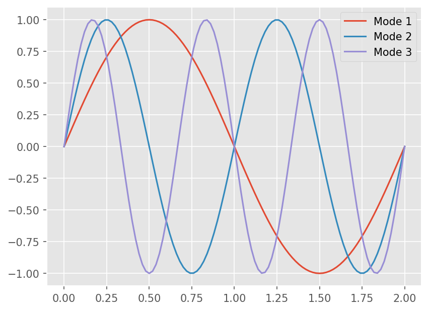
for i in range(1, 4):
plt.plot(x, np.sin(np.pi*i*x))
legends.append("Mode {}".format(i))
plt.legend(legends)
<matplotlib.legend.Legend at 0xff05a98b9390>
Modified wavenumber
간단한 Harmonic 함수에 대해 분석
\[ f(x) = e^{ikx}, \]\([0, L]\) 영역을 N개의 격자로 나누었다고 생각하자. 이때 waveumber \(k\)를 다음과 같이 고려하자
\[ k = \frac{2\pi}{L} n, ~~~n=0, 1, 2, ... \frac{N}{2} \]이론적인 미분은
\[ f' = ikf \]Finite difference
격자점은
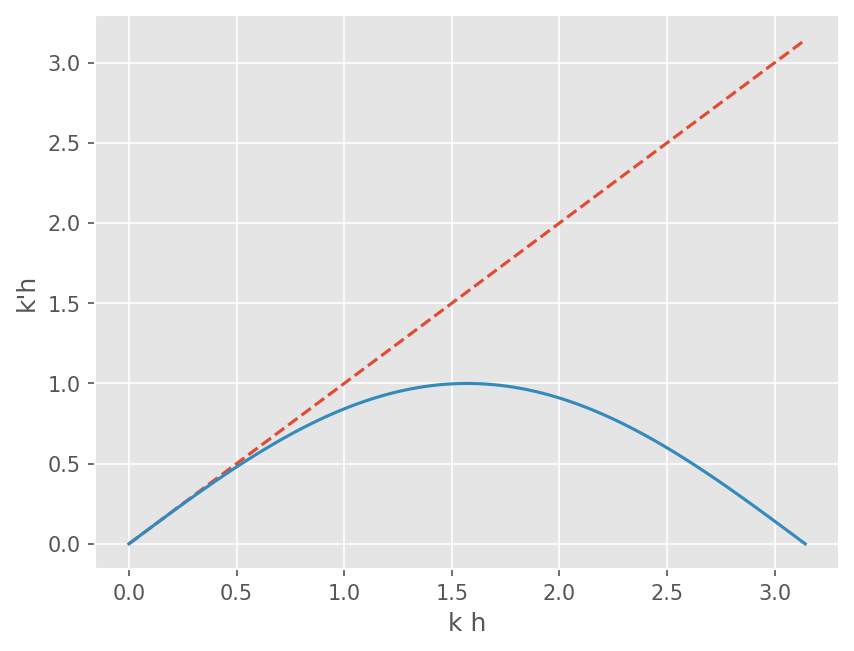
\[ x_j = \frac{L}{N} j ~~~j=0,1,2,...,N. \]Central differnce에 대해 Harmonic 함수 적용
\[ f'_j = f'(x_j) = \frac{f(x_{j+1}) - f(x_{j-1})}{2\Delta x} = \frac{e^{i 2\pi n (j+1)/N} - e^{i 2\pi n (j-1)/N}}{2\Delta x} = \frac{e^{i 2\pi n /N} - e^{-i 2\pi n /N}}{2\Delta x} f_j \]\[ f'_j = i \frac{\sin(2\pi n/N)}{\Delta x} f_j = ik'f_j \]즉
\[ k' \Delta x = \sin(2\pi n/N) = \sin (k \Delta x) \]
kh = np.linspace(0, np.pi, 101)
mkh = np.sin(kh)

plt.plot(kh, kh, linestyle='--')
plt.plot(kh, mkh)
plt.xlabel('k h')
plt.ylabel("k'h")
Text(0, 0.5, "k'h")
def forward_diff(f, x, dx):
# Forward difference
return (f(x+dx) - f(x)) / dx
def backward_diff(f, x, dx):
# Backward difference
return (f(x) - f(x-dx)) / dx
def central_diff(f, x, dx):
# Central difference
return (f(x+dx) - f(x-dx)) / (2*dx)
def compute(dx):
x = np.linspace(0, 2*np.pi, 101)
f = np.sin
# Compute first derivatives
exact = np.cos(x)
fd = np.array([forward_diff(f, xi, dx) for xi in x])
bd = np.array([backward_diff(f, xi, dx) for xi in x])
cd = np.array([central_diff(f, xi, dx) for xi in x])
return x, exact, fd, bd, cd
def plot(dx):
x, exact, fd, bd, cd = compute(dx)
# Plot
plt.plot(x , exact)
plt.plot(x, fd)
plt.plot(x, bd)
plt.plot(x, cd)
plt.legend(['Exact', 'Forward Difference', 'Backward Difference', 'Central Difference'])
plt.xlabel(r'x')
plt.ylabel(r"$f'(x)$")
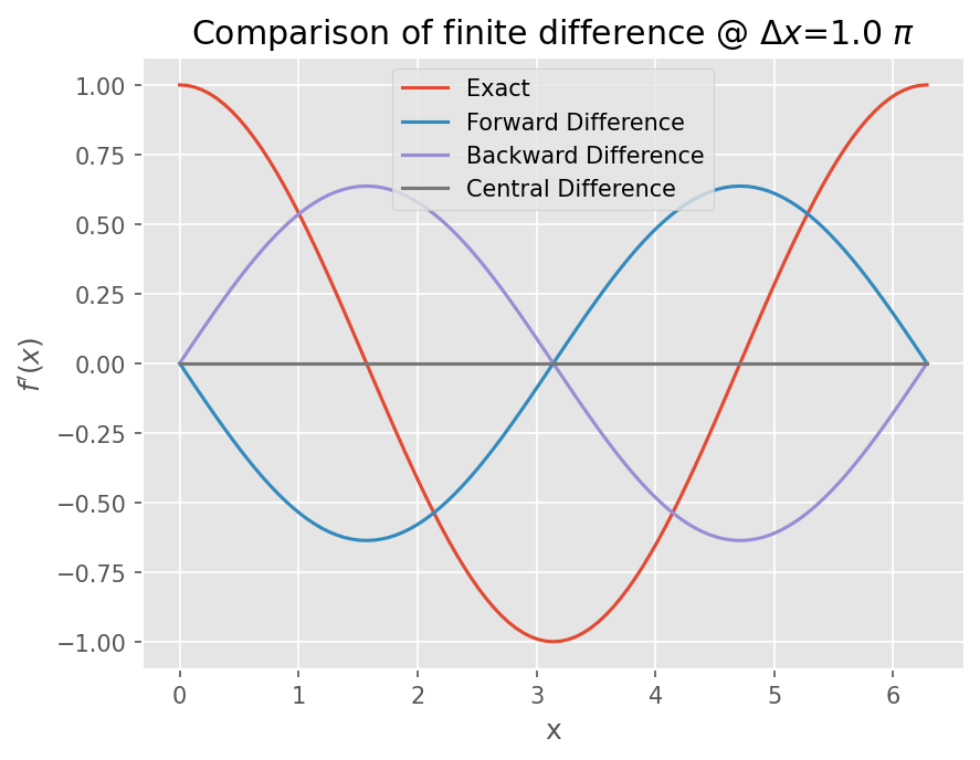
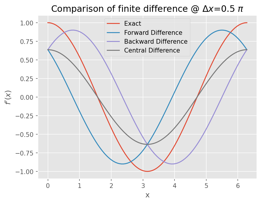
plt.title("Comparison of finite difference @ $\Delta x$={} $\pi$".format(dx/np.pi))
plot(0.5*np.pi)
plot(np.pi)